6.5 Chain matrix multiplication

6.5 Chain matrix multiplication

Suppose that we want to multiply four matrices, $A\times B\times C\times D$ , of dimensions $50\times 20,20\times 1$ $1\times 10,$ , and $10\times 100$ , respectively (Figure 6.6). This will involve iteratively multiplying two matrices at a time. Matrix multiplication is not commutative (in general, $A\times B\ne B\times A)$ , but it is associative, which means for instance that $A\times (B\times C)=(A\times B)\times C$ . Thus we can compute our product of four matrices in many different ways, depending on how we parenthesize it. Are some of these better than others?

Multiplying an $m\times n$ matrix by an $n\times p$ matrix takes mnp multiplications, to a good enough approximation. Using this formula, let’s compare several different ways of evaluating $A\times B\times C\times D$

Parenthesization	Cost computation	Cost
$A\times ((B\times C)\times D)$	$20\cdot 1\cdot 10+20\cdot 10\cdot 100+50\cdot 20\cdot 100$	120,200
$(A\times (B\times C))\times D$	$20\cdot 1\cdot 10+50\cdot 20\cdot 10+50\cdot 10\cdot 100$	60,200
$(A\times B)\times (C\times D)$	$50\cdot 20\cdot 1+1\cdot 10\cdot 100+50\cdot 1\cdot 100$	7,000

As you can see, the order of multiplications makes a big difference in the final running time! Moreover, the natural greedy approach, to always perform the cheapest matrix multiplication available, leads to the second parenthesization shown here and is therefore a failure.

How do we determine the optimal order, if we want to compute $A_1\times A_2\times \cdots \times A_n,$ , where the $A_i\dot{\mathbf{s}}$ are matrices with dimensions $m_0\times m_1,m_1\times m_2,\dots ,m_{n-1}\times m_n$ , respectively? The first thing to notice is that a particular parenthesization can be represented very naturally by a binary tree in which the individual matrices correspond to the leaves, the root is the final product, and interior nodes are intermediate products (Figure 6.7). The possible orders in which to do the multiplication correspond to the various full binary trees with n leaves, whose

overline text Figure 6.7(a) ((A × B) × C) × D ; (mathbf b) A × ((B × C) × D) ; (mathbf c) (A × (B × C)) × D .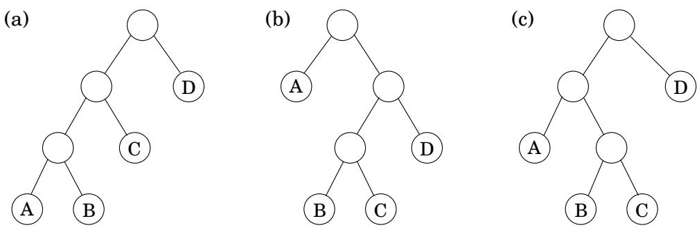$$\overline{\text{ Figure 6.7(a) }((A\times B)\times C)\times D;(\mathbf{b})A\times ((B\times C)\times D);(\mathbf{c})(A\times (B\times C))\times D.}$$

number is exponential in n (Exercise2.13). We certainly cannot try each tree, and with brute force thus ruled out, we turn to dynamic programming.

The binary trees of Figure 6.7 are suggestive: for a tree to be optimal, its subtrees must also be optimal. What are the subproblems corresponding to the subtrees? They are products of the form $A_i\times A_{i+1}\times \cdots \times A_j$ . Let’s see if this works: for $1\le i\le j\le n$ , define

C (i, j) = text minimum cost of multiplying A _ i × A _ i + 1 × … × A _ j.$$C(i,j)=\text{ minimum cost of multiplying }{A}_i\times A_{i+1}\times \cdots \times A_j.$$

The size of this subproblem is the number of matrix multiplications, $|j-i|$ The smallest subproblem is when $i=j,$ , in which case there’s nothing to multiply, so $C(i,i)=0$ . For $j>i,$ consider the optimal subtree for $C(i,j)$ . The first branch in this subtree, the one at the top, will split the product in two pieces, of the form $A_i\times \cdots \times A_k$ and $A_{k+1}\times \cdots \times A_j$ , for some k between i and $j.$ . The cost of the subtree is then the cost of these two partial products, plus the cost of combining them: $C(i,k)+C(k+1,j)+m_{i-1}\cdot m_k\cdot m_j$ . And we just need to find the splitting point k for which this is smallest:

C (i, j) = min _ i ≤ k < j {C (i, k) + C (k + 1, j) + m _ i - 1 · m _ k · m _ j }.$$C(i,j)=\underset{i\le k<j}{\min }\left\{C(i,k)+C(k+1,j)+m_{i-1}\cdot m_k\cdot m_j\right\}.$$

We are ready to code! In the following, the variable s denotes subproblem size.

l text for i = 1 to n: C(i,i) = 0 text for s = 1 to n - 1: text for i = 1 to n - s: j = i + s C (i, j) = min {C (i, k) + C (k + 1, j) + m _ i - 1 · m _ k · m _ j: i ≤ k < j } text return C(1,n)$$\begin{array}{l}\text{for i = 1 to n: C(i,i) = 0}\\ \text{for s = 1 to n - 1:}\\ \text{for i = 1 to n - s:}\\ j=i+s\\ C(i,j)=\min \{C(i,k)+C(k+1,j)+m_{i-1}\cdot m_k\cdot m_j:i\le k<j\}\\ \text{return C(1,n)}\end{array}$$

The subproblems constitute a two-dimensional table, each of whose entries takes $O(n)$ time to compute. The overall running time is thus $O(n^3)$