2.2 Recurrence relations

2.2 Recurrence relations

Divide-and-conquer algorithms often follow a generic pattern: they tackle a problem of size n by recursively solving, say, a subproblems of size $n/b$ and then combining these answers in $O(n^d)$ time, for some $a,b,d>0$ (in the multiplication algorithm, $a=3,b=2,$ , and $d=1)$ . Their running time can therefore be captured by the equation $T(n)=aT(\lceil n/b\rceil )+O(n^d)$ . We next derive a closed-form solution to this general recurrence so that we no longer have to solve it explicitly in each new instance.

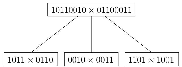
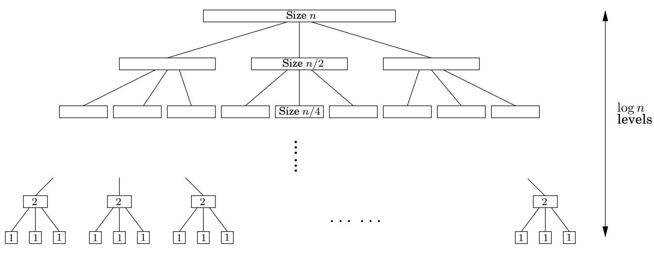
Figure 2.2 Divide-and-conquer integer multiplication. ($a$) Each problem is divided into three subproblems. ($b$) The levels of recursion.

($a$)

($b$)

Master theorem² $IfT(n)=aT(\lceil n/b\rceil )+O(n^d)$ for some constants $a>0,b>1$ and $d\ge 0.$ then

T (n) = { l l O (n ^ d) & text if d > log_ b a O (n ^ d log n) & text if d = log_ b a O (n ^ log_ b a) & text if d < log_ b a. .$$T(n)=\{\begin{array}{ll}O(n^d)& \text{if}d>{\log }_{b}a\\ O(n^d\log n)& \text{if}d={\log }_{b}a\\ O(n^{{\log }_{b}a})& \text{if}d<{\log }_{b}a.\end{array}$$

This single theorem tells us the running times of most of the divide-and-conquer procedures we are likely to use.

Proof

To prove the claim, let’s start by assuming for the sake of convenience that n is a power of $b.$ This will not influence the final bound in any important way—after all, n is at most a multiplicative factor of b away from some power of b (Exercise2.2)—and it will allow us to ignore the rounding effect in $\lceil n/b\rceil$

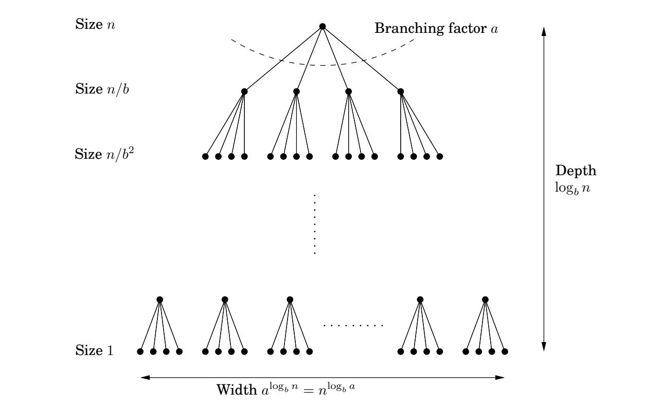
Next, notice that the size of the subproblems decreases by a factor of b with each level of recursion, and therefore reaches the base case after ${\log }_{b}n$ levels. This is the height of the recursion tree. Its branching factor is ${}^{a,}$ so the kth level of the tree is made up of $a^k$ subproblems, each of size $n/b^k$ (Figure 2.3). The total work done at this level is

Figure 2.3 Each problem of size n is divided into a subproblems of size $n/b.$

a ^ k × O (frac nb ^ k) ^ d = O (n ^ d) × (frac ab ^ d) ^ k.$$a^k\times O{\left(\frac{n}{b^k}\right)}^d=O(n^d)\times {\left(\frac{a}{b^d}\right)}^k.$$

As k goes from 0 (the root) to ${\log }_{b}n$ (the leaves), these numbers form a geometric series with ratio $a/b^d$ . Finding the sum of such a series in big-O notation is easy (Exercise0.2), and comes down to three cases.

1. The ratio is less than 1.

Then the series is decreasing, and its sum is just given by its first term, $O(n^d)$

2. The ratio is greater than 1.

The series is increasing and its sum is given by its last term, $O(n^{{\log }_{b}a})$

n ^ d (frac ab ^ d) ^ log_ b n = n ^ d (frac a ^ log_ b n(b ^ log_ b n) ^ d) = a ^ log_ b n = a ^ (log_ a n) (log_ b a) = n ^ log_ b a.$$n^d{\left(\frac{a}{b^d}\right)}^{{\log }_{b}n}=n^d\left(\frac{a^{{\log }_{b}n}}{(b^{{\log }_{b}n}{)}^d}\right)=a^{{\log }_{b}n}=a^{({\log }_{a}n)({\log }_{b}a)}=n^{{\log }_{b}a}.$$

3. The ratio is exactly 1.

In this case all $O(\log n)$ terms of the series are equal to $O(n^d)$

These cases translate directly into the three contingencies in the theorem statement.

Box: Binary search

The ultimate divide-and-conquer algorithm is, of course, binary search: to find a key k in a large file containing keys $z[0,1,\dots ,n-1]$ in sorted order, we first compare k with $z[n/2]$ , and depending on the result we recurse either on the first half of the file, $z[0,\dots ,n/2-1]$ , or on the second half, $z[n/2,\dots ,n-1]$ . The recurrence now is $T(n)=T(\lceil n/2\rceil )+O(1)$ , which is the case $a=1,b=2,d=0.$ Plugging into our master theorem we get the familiar solution: a running time of just O(log n).